
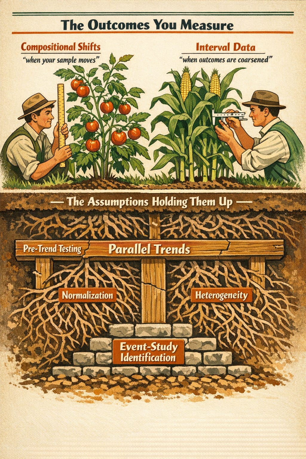
The outcomes you measure and the assumptions holding them up
New papers on compositional shifts, coarsened outcomes, pre-trend testing and event-study identification

Hi there!
Thank you (all 1553 of you) for being here for one year now :)
I wanted to close 2025 with a “banger” - meaning lots of banger papers - but I got distracted by the only 2 weeks I have of free-time in the year. Apologies. Also I am set to graduate in May while also teaching a course this term, so probably the rate of posts will come down just a bit, but after May it should resume to normal.
Here’s to many more posts in 2026 :)
Also before we get to the papers, I’d like to thank my friend Sam Enright who picked 3 posts from this newsletter for The Fitzwilliam Reading Group monthly meetup a couple of weeks ago. Special thanks to those who attended and who are reading this now :)
As always, please let me know if you would like for me to cover a specific paper. I will do my best to go through it.
Today’s papers are:
Difference-in-Differences with Compositional Changes, by Pedro H. C. Sant’Anna and Qi Xu
Difference-in-Differences with Interval Data, by Daisuke Kurisu, Yuta Okamoto and Taisuke Otsu
Testing for equivalence of pre-trends in Difference-in-Differences estimation, by Holger Dette and Martin Schumann
Harvesting Difference-in-Differences and Event-Study evidence, by Alberto Abadie, Joshua Angrist, Brigham Frandsen and Jörn-Steffen Pischke
Honorable mention:
Synthetic Parallel Trends, by Yiqi Liu
Difference-in-Differences with Compositional Changes
TL;DR: standard DiD with repeated cross-sections relies on a strong stationarity assumption that often fails in practice. Sant’Anna and Xu show that the ATT remains identifiable when composition shifts, derive the correct efficiency bound and provide robust estimators and a diagnostic test to assess whether stationarity is empirically relevant. The paper formalises the bias–variance trade-off and gives applied researchers a clear framework for working with moving samples.
What is this paper about?
This paper is about a quite strong and often unrealistic (in practice) assumption in DiD with repeated cross-sections1: no compositional changes over time, which means assuming that the treated and control groups come from the same underlying population before and after treatment. In many real applications this is straight implausible: people enter and leave samples, early adopters differ from late adopters, firms exit, migrants move, and survey frames rotate. This is the default setting for many labour, health, education and dev applications that rely on repeated survey data.
A classic example cited by the authors is the study of Napster’s effect on music sales. Over time, the composition of internet users changed substantially: early adopters were typically younger and wealthier while later adopters were more demographically diverse. If a researcher ignores these shifts, the negative effect of Napster on sales might be overestimated because the “post-Napster” group naturally includes more households with lower reservation prices for music, regardless of the technology’s impact.
Most DiD methods simply impose stationarity2 and move on. Sant’Anna and Xu do the opposite. They study DiD when composition is allowed to change and show that the ATT remains identifiable under conditional PT3. They develop a general framework that makes clear what is identified, at what cost in efficiency, and how standard approaches break down when compositional changes are ignored.
What do the authors do?
They start by dropping the usual stationarity assumption and allowing the joint distribution of (D,X) to change over time. In this setup, they show that the ATT is still identified under conditional PT, no anticipation, and overlap. However, the “math” changes: because you can no longer assume the population is stable, you have to track four distinct groups (treated/control in both periods) using a generalized propensity score.
They derive the efficient influence function (EIF) and efficiency bound4 (essentially the “gold standard” for precision) for the ATT when composition is allowed to shift, and build nonparametric doubly robust5 estimators that remain valid under these compositional shifts. Unlike classical DR, which relies on getting one of two models “correct”, their estimators enjoy a rate doubly robust property. This means your estimate is reliable even if one part of your model (like the outcome regression) is very complex, provided the other part (the propensity score) is simple enough to compensate. They prove that the widely used Sant’Anna–Zhao (2020) estimator can be biased because it wasn’t designed to handle these moving populations.
They then characterize the bias–variance trade-off. If you wrongly impose stationarity, you can get biased ATT estimates. If you don’t impose it when it actually holds, you lose efficiency. You might be attributing a change in the data to the treatment when it’s actually just a result of the “mix” of people in your sample changing. However, robustness isn’t free. If stationarity really holds but you choose to ignore it by using the robust estimator, you lose efficiency (precision). Proposition 2.2 identifies three factors that determine how much precision you lose: the period ratio (the balance between the size of your pre-treatment and post-treatment sample; the group ratio (the proportion of comparison units relative to treated units; and treatment heterogeneity (aka how much the treatment effect varies across different types of people). In a world where everyone responds to a policy in exactly the same way (homogeneous effects), the robust estimator is just as precise as the standard one. In the real world, where effects usually vary, the test they propose becomes your essential “GPS” for navigating this trade-off.
To operationalise this, they propose a Hausman-type test6 that compares the robust estimator (valid under compositional changes) with the stationarity-based estimator. The idea is simple: if composition doesn’t matter for the ATT, the two should coincide; if they differ, stationarity is empirically relevant. This concentrates power exactly in the directions that matter for the target parameter.
Then they show how to implement all of this in practice. They use local polynomial methods for outcome regressions and local multinomial logit for generalized propensity scores, allow for both continuous and discrete covariates, discuss bandwidth selection, extend the framework to cross-fitting and mixed panel/cross-section designs, and illustrate the methods in simulations and an application.
Why is this important?
Many applied DiD papers rely on repeated cross-sections and proceed under an implicit stationarity assumption. This paper shows that this choice has real consequences for identification and precision. When composition changes, standard DiD estimators can be biased even if conditional PT holds. This affects the credibility of causal claims in a wide range of applications, as researchers might mistake a demographic shift for a policy effect.
The contribution here is diagnostic as much as methodological. Sant’Anna and Xu show exactly where the bias comes from, how large it can be and which assumptions remove it. This replaces hand-waving about “changing samples” with a precise link between assumptions, estimands and estimators.
The bias–variance trade-off is very important for practice. Imposing stationarity “buys” precision at the cost of bias when the assumption fails. Dropping it “buys” robustness at the cost of efficiency when the assumption holds. The paper formalises this trade-off and provides a test to decide which side you’re on. This then gives applied researchers a way to justify their design choices rather than rely on convention.
More broadly, the paper aligns DiD theory with how data are generated. Repeated cross-sections aren’t panels. Populations evolve. Treating moving samples as if they were fixed is convenient, but often inaccurate. By building the theory for the setting we actually face, this paper closes an important gap between methodological assumptions and empirical practice.
Who should care?
Applied researchers using DiD with survey or administrative data should pay attention. This includes work in labour, health, education, development and public policy where repeated cross-sections are the norm. Those using repeated cross-sectional data from major national sources like the Current Population Survey (CPS) or the Consumer Expenditure Survey (CEX). If your identification strategy relies on treating moving samples as stable groups, this paper speaks directly to your design choices.
Policy evaluators working on national reforms, programme expansions or regulatory changes are another core audience. In many of these settings, the underlying population evolves at the same time as the policy environment. The framework here clarifies when standard DiD logic carries through and when different estimators are needed, which is directly relevant for government analysts and policy units producing causal evidence under real-world constraints.
Methodologically, this paper will be useful for researchers building or using modern DiD estimators. It tightens the link between assumptions, estimands and efficiency, and shows how robustness to compositional change interacts with precision. If you work with DR methods, semiparametric efficiency or ML in DiD, the technical contributions here are relevant.
Referees and editors should also care. Many papers implicitly rely on stationarity without stating it. This paper provides language and tools to assess that assumption rather than take it on faith which raises the bar for what we can reasonably claim in applied work.
Do we have code?
Not in the paper itself. While no dedicated software package is listed, the authors provide the exact mathematical estimators in Section 3. They recommend using local polynomial and multinomial logit tools, which are available in general-purpose R packages like np or npsf, and then combining them according to the ATT formula derived in the paper. Check Supplemental Appendix for implementation, where they give a practical recipe (local polynomial outcome regressions + local multinomial logit generalised propensity scores + cross-validation/bandwidth choices), but you’d code it yourself (or adapt existing nonparametric/kernel + multinomial logit tooling).
In summary, this great paper revisits DiD with repeated cross-sections. Sant’Anna and Xu show that the ATT remains identifiable under conditional PT, but the estimand, efficiency bound and appropriate estimator change once stationarity is dropped. They derive the efficient influence function, build rate DR estimators that remain valid under shifting composition and make the bias–variance trade-off explicit. The Hausman-type test gives applied researchers a way to assess whether stationarity is empirically relevant rather than assume it. Overall, the paper replaces a convenient convention with a clear design framework and provides tools that align DiD practice with how samples evolve in reality.
Difference-in-Differences with Interval Data
(Yuta is a 3rd-year PhD student at the Graduate School of Economics, Kyoto University)
TL;DR: traditional DiD assumes scalar (exact) outcomes, but real-world data is often “coarsened” into intervals through rounding or binned reporting. The authors demonstrate that instead of naively extending “parallel trends”, a “parallel shifts” assumption is necessary to ensure the resulting bounds are both mathematically valid and intuitively sensible. Through their reanalysis of the Card and Krueger (1994) study, they show that this new method provides a more disciplined and informative way to handle rounding and heaping in employment data.
What is this paper about?
This paper is about a problem almost nobody talks about in DiD: what happens when your outcome isn’t a number, but an interval. In a lot of survey and administrative data, outcomes are reported in brackets, bins or rounded chunks. Income, e.g., is a range. Hours worked are heaped at multiples of five. Headcounts are approximate. Even when datasets look scalar, they often aren’t, because rounding, heaping and reporting conventions mean the “true” value sits somewhere inside an interval. In this paper, Kurisu, Okamoto, and Otsu tell us to reconsider our choices. They ask: how should we do difference-in-differences when outcomes are interval-valued rather than point-valued? And more importantly: what does “parallel trends” even mean in that world?
Their first result is quite uncomfortable: if you naively apply the PT assumption to interval data, you can get bounds that are either so wide they’re useless, or that move in directions that make no sense. You can satisfy “parallel trends” and still get counterintuitive or uninformative results.
So the paper’s core contribution is conceptual. It shows that extending PT to interval outcomes is not without a cost, and that you need a different way of thinking about how treated and control groups should evolve over time. The authors propose an alternative assumption - parallel shifts - that’s designed to respect how intervals move and scale, and to avoid the pathologies that show up under naïve extensions.
What do the authors do?
They set up DiD properly for interval data. Instead of observing a single outcome, each unit is observed as a lower and an upper bound. The target is still the ATT, but now both the treated mean and the counterfactual mean are only partially identified.
They then study three ways of bringing PT into this setting. First, they apply standard PT to the unobserved true outcome. This is the most direct extension of textbook DiD. It performs badly. The bounds are extremely wide and often dominated by worst-case combinations of lower and upper bounds across groups.
Second, they apply PT directly to the interval bounds, that is, they track how the control group’s lower and upper bounds change over time and project those changes onto the treated group. This looks intuitive, but it can behave in strange ways. You can end up with treated bounds moving in the opposite direction to control bounds, even though “parallel trends” is imposed.
They then propose a different assumption: parallel shifts. Instead of matching trends over time, it matches shifts between groups. The idea is that whatever mapping takes the control group’s interval to the treated group’s interval before treatment is assumed to also apply after treatment. Under this assumption, the bounds move in the same direction across groups, interval widths behave sensibly, and the identified sets remain well-behaved. They derive closed-form bounds for the ATT so the method is easy to implement.
Finally, they apply the framework to the C&K minimum wage study, treating employment as interval-valued because of rounding and heaping, and show how the different assumptions lead to very different conclusions.
Why is this important?
Because the way outcomes are recorded affects what DiD can identify.
In many survey and administrative datasets, outcomes are reported in brackets, rounded, or subject to heaping. Income is often binned. Hours worked cluster at focal values. Headcounts are approximate. In these settings, the outcome is a range rather than a point.
The standard DiD framework treats outcomes as exact and applies PT to their means. This paper shows that once outcomes are interval-valued, that logic does not carry over in a clear way. Some natural ways of extending PT lead to bounds that are very wide or that move in ways that are difficult to justify, which has direct consequences for interpretation. With the same data, different extensions of PT can produce very different identified sets. The identifying assumptions are doing more work than is usually acknowledged.
The contribution of the paper is to make that structure explicit. It shows that transporting information from control to treated is not neutral when outcomes are coarsened, and that some ways of doing it behave better than others. The parallel shifts assumption is proposed as a disciplined way of mapping intervals across groups and over time.
More broadly, the paper sits in the partial identification space. Once outcomes are coarsened, point identification is no longer guaranteed. Bounds are often the appropriate object. That is less convenient, but it reflects the information in the data.
Who should care?
Researchers using DiD with survey or administrative data where outcomes are coarsened. This includes work on income, wages, hours worked, employment, firm size, time use, and test scores when these are reported in brackets, rounded, or subject to heaping. It is common in labour, health, education, and public policy applications.
It is also relevant for people working with repeated cross-sections. In these settings, binning and rounding are standard, and the choice to treat midpoints as exact values is widespread. This paper shows that those choices have identifying consequences.
More broadly, anyone interested in identification in DiD, rather than only estimation, will find this useful. The paper makes clear that different ways of extending PT are not equivalent once outcomes are interval-valued. It is also relevant for readers working on partial identification and bounded inference. The framework fits well in settings where point identification is not credible.
Do we have code?
The paper derives closed-form bounds, so implementation is should be more or less straightforward. Everything is based on sample means of observed lower and upper bounds, with no optimisation or simulation required. Reproducing the results should be easy in R, Stata, or Python. The authors don’t provide replication code with the paper. The C&K reanalysis uses standard data and simple transformations, so I think we could reconstruct it. If you are planning to use this in practice, you will need to code it yourself.
In summary, this paper asks what DiD is really doing when outcomes are interval-valued rather than exact. It shows that standard ways of extending PT can produce wide or poorly behaved bounds. The authors propose an alternative assumption, parallel shifts, that maps intervals across groups in a more disciplined way and leads to well-behaved identified sets. The contribution is conceptual. It makes clear that once outcomes are coarsened, identification depends heavily on how structure is imposed. Different choices lead to different answers. If your outcomes are rounded, binned, or heaped, this paper is directly relevant.
Testing for equivalence of pre-trends in Difference-in-Differences estimation
TL;DR: we test the wrong thing when we check pre-trends in DiD. The usual null is “no difference”. Failing to reject is then treated as evidence for PT. The authors say that logic is weak: it often means the data say nothing. In large samples it can reject for tiny, irrelevant differences. This paper proposes equivalence tests instead. You test whether pre-trend differences are small enough to ignore. The null is that they are too large. Rejection gives actual support for the identifying assumption.
What is this paper about?
This paper is about how we test the PTA in DiD. In applied work, the standard approach is to test whether pre-treatment differences between treated and control groups are statistically zero. If you fail to reject, you proceed. The authors argue this logic is backwards. Failing to reject zero doesn’t mean trends are similar. It often means the test has low power. In large samples, the same tests can reject for tiny, irrelevant differences. Either way, the usual pre-tests do not answer the question practitioners actually care about.
The paper proposes replacing “no difference” tests with equivalence tests. Instead of asking whether pre-trends are exactly the same, it asks whether any differences are small enough to be considered negligible. The null becomes “differences are non-negligible”. Rejection then gives positive evidence in favour of PT.
The core object here is the size of pre-treatment trend differences, and whether the data support treating them as effectively zero for identification. The paper is about formalising that logic and giving tools to implement it.
What do the authors do?
They formalise pre-trend checking as an equivalence testing problem. Instead of testing whether each pre-treatment coefficient is zero, they define null hypotheses where pre-trend differences are at least as large as a user-chosen threshold. The alternative is that all differences are smaller than that threshold. Rejection then gives evidence that deviations from PT are negligible.
They propose three ways to summarise pre-trend differences: the maximum deviation across periods, the average deviation, and the root mean square deviation. Each corresponds to a different notion of what “small enough” means. The choice is left to the researcher and should be justified in context. They develop test statistics for each case, show their asymptotic properties and discuss implementation. In practice this means estimating the usual pre-treatment coefficients, then testing whether their joint behaviour stays within the chosen bound. They also show how to recover the smallest threshold for which equivalence would be accepted, if the researcher does not want to commit to a bound ex ante.
They extend the framework to staggered adoption and heterogeneous treatment effects using regression-based DiD setups. The idea is the same: define placebo effects in pre-treatment periods and test whether those are jointly small.
They back this up with simulations and an empirical illustration. The simulations compare equivalence tests to standard pre-tests under different violations of PT. The application re-examines a well-known DiD study and shows that, under their approach, the data give weak support for treating pre-trends as negligible.
Why is this important?
This is important because the usual pre-trend checks do not answer the identification question we are pretending they answer. In DiD, PT is an assumption, we never observe the counterfactual. Pre-trend tests are meant to give reassurance that the assumption is plausible, but the standard null is “no difference”. Failing to reject that null is often read as evidence of similarity. That is a logical error. It usually means the data are uninformative. This then creates two problems. In small samples, you can have meaningful differences in trends that go undetected. In large samples, you can reject for tiny differences that are irrelevant for the treatment effect. In both cases, the test result is hard to interpret for identification.
Equivalence testing flips the burden of proof. The null is that differences are large enough to worry about. To proceed, the data must show that differences are smaller than a threshold you consider acceptable. That aligns the test with the actual identifying assumption. You are no longer asking whether trends are identical, but rather whether deviations are small enough that treating them as zero is defensible.
This also forces structure. You have to say what “small enough” means in your application. That makes the identifying assumptions explicit rather than implicit. If you can’t justify any threshold, you can report the smallest one the data would support. That gives a direct sense of how much non-parallelism is compatible with your design. From an applied perspective, this changes interpretation. Instead of “we don’t see pre-trends”, you get “the data support ruling out pre-trend differences larger than X”. That is a statement about identification strength, not about p-values.
Who should care?
Everyone. We all do pre-trend checks. They sit at the start of almost every DiD design. They are usually the first thing people look at and the first thing readers use to judge credibility. This paper is about that step. The first one in the default workflow.
If you run event studies, plot leads, or report placebo regressions to justify PT, this applies to you. The argument is that the usual logic behind those checks is weak and often misleading. Equivalence testing is a way to make that step mean what we pretend it means.
This includes work with small samples, short panels, survey data, administrative data, and everything in between. It includes clean policy designs and messy real-world ones. If PT is doing identifying work in your paper, this framework is relevant.
Do we have code?
In a narrow sense, yes. The simulations are implemented in R and the empirical illustration is fully reproducible. The paper describes the procedures in enough detail that replication is straightforward, and the authors indicate that code is available. There is no standalone package or user-friendly wrapper. This is not a plug-and-play tool. That is consistent with the paper’s aim. The contribution is conceptual and inferential. If you’re comfortable writing your own pre-trend regressions and working with bootstrap routines, you can implement these tests without much friction. If you are not, there is no ready-made function you can drop into your workflow so maybe wait a little?
In summary, this paper is about aligning pre-trend checks with what PT means for identification. The standard workflow tests whether pre-treatment differences are zero, but that’s not the question we care about. We care whether differences are small enough to ignore. The authors show how to formalise that directly, using equivalence tests that put the burden of proof where it belongs. Their contribution is a way of being honest about assumptions: you either justify a threshold for negligible differences or you report how large differences could be before the design breaks. In both cases, interpretation improves. If you take PT seriously as an identifying restriction, this is a cleaner way to assess it.
Harvesting Difference-in-Differences and Event-Study evidence
TL;DR: this paper dissects what modern DiD and event-study workflows are really identifying, using a single policy setting to show how normalisation, heterogeneity and design choices shape the estimand. It shows that dynamic paths, exposure coefficients and pre-trend checks carry more identifying content than many of us realise, and that regression output is often easier to compute than to interpret. The message is that standard implementations impose structure that is rarely acknowledged. If you use event studies or exposure designs, this paper sharpens the link between your code and your causal claims.
What is this paper about?
This paper is a guided walk through modern DiD and event-study practice, it’s a synthesis and critique of what people are actually doing with staggered adoption, dynamic effects, exposure designs and pre-trend checks.
The authors use the unilateral divorce reforms in US states as a running example. They use it to show how static DiD, event studies and newer heterogeneity-robust approaches behave in practice. Their focus is on interpretation rather than technique, what is being identified under which assumptions, and how easy it is to get something that looks clean but is hard to interpret.
Three themes run through the paper. First, normalisation isn’t harmless in event studies because when and how you anchor the coefficients can change the shape of the estimated dynamics. Second, heterogeneous and time-varying effects complicate both static DiD and event-study estimates. The paper is explicit about where regression averages do and do not correspond to meaningful causal objects. Third, common workflow steps like pre-trend testing and log specifications carry stronger identifying content than many of us realise.
The paper’s goal is rather practical. It’s a great attempt at trying to discipline how we read DiD and event-study output, what object is this coefficient estimating, which assumptions are doing the work, and where the usual visual and statistical checks can mislead.
What do the authors do?
They take a single policy setting and run it through the full modern DiD toolkit: static two-way fixed effects, event studies with leads and lags, alternative normalisations, heterogeneity-robust approaches, exposure designs, pre-trend testing, and logs versus levels. The unilateral divorce reforms are the running example, used to illustrate how identification and interpretation change across specifications.
They start from the canonical TWFE model and make the identifying assumptions explicit: additive state and time effects +PT in untreated potential outcomes + no anticipation. They then introduce event-time indicators to allow for dynamic effects and show how this immediately creates normalisation problems. With staggered adoption and no never-treated units, at least two coefficients must be set to zero. Which ones you choose changes the shape of the estimated path.
They then move to treatment effect heterogeneity. First in simple two-period settings, where TWFE still recovers an average effect under clear conditions, then in staggered designs with dynamic effects, where already-treated units act as controls and regression averages can become hard to interpret. Small numerical examples are used to show when static DiD collapses and when event studies produce misleading dynamics.
For exposure designs, they write down a model where treatment is continuous rather than binary and allow effects to vary with exposure intensity. They show that the usual regression coefficient identifies an average marginal effect, not an average of underlying treatment effects. This distinction is carried through using the potato example.
They also implement the BJS imputation estimator on the divorce data and compare it to standard event-study regressions. This is used to assess how much cross-sectional heterogeneity actually distorts regression-based dynamics in a real application.
At the end they examine pre-trend testing and inference, discuss why lead coefficients are a pre-test, why this can create problems for inference and why it is still informative in practice. They also simulate clustered standard errors in staggered event studies to show how leverage and limited treated observations at long horizons can understate uncertainty.
Why is this important?
A large share of applied DiD and event-study work relies on regression output that looks intuitive but is tightly tied to modelling choices that are rarely spelled out, and this paper shows in a very concrete way where structure is being imposed and how that structure shapes what is being identified. Normalisation choices in event studies are not cosmetic. Using already-treated units as controls is not neutral. Exposure designs are not estimating the same object as binary DiD. Lead coefficients are not just informal diagnostics. Each of these decisions changes the estimand, often in ways that are easy to miss when reading a table or a plot.
The paper is also important because it forces some discipline into how we talk about dynamics and heterogeneity. Many applied papers present event-time paths, average effects and pre-trend plots as if they were direct summaries of the data, when in fact they are products of models that restrict untreated potential outcomes, restrict how treatment effects evolve over time and restrict how heterogeneity enters. Once those restrictions are written down, it becomes much harder to treat the output as self-explanatory.
The exposure design discussion makes this very clear. A single regression coefficient is often read as “the effect of exposure”, but in the presence of heterogeneity it is an average marginal effect, not an average of underlying treatment effects, and those two objects diverge as soon as effects vary with exposure intensity. That is an interpretation problem and it applies directly to a large class of shift-share and intensity-based designs.
The same logic applies to event studies. When there are no never-treated units, at least two coefficients are pinned down by assumption rather than data, and with heterogeneous effects the estimated dynamics can reflect changing composition of contributing units rather than changes in causal impacts. None of this requires pathological designs. It arises in settings that look standard.
On pre-trends and inference, the paper is explicit about trade-offs that are often waved away. Lead coefficients are pre-tests. Pre-tests affect post-test interpretation. Clustered standard errors behave poorly when only a few units identify long leads and lags. These are features of the designs we actually use.
Overall, the value of the paper is that it tightens the link between regression output and causal interpretation in a way that is directly relevant for applied work. It keeps bringing the reader back to the same questions: what is being identified, under which assumptions, and whether that object matches the story being told.
Who should care?
Anyone running DiD or event studies in applied work, which in practice means most people doing policy evaluation with panel or repeated cross-section data. If you use staggered adoption, plot leads and lags, average dynamic effects, or rely on pre-trend checks to support identification, this paper is written for you.
This includes people working with clean administrative panels and people working with short, noisy surveys. It includes settings with clear policy shocks and settings with fuzzy timing. It includes binary treatments and exposure designs. The issues the paper raises are not niche. They show up in default workflows.
It is also relevant for readers and referees. If you are judging whether an event-study plot support PT, whether a dynamic path is meaningful, or whether an exposure coefficient has a sensible interpretation, the paper gives you a sharper set of questions to ask. Where is the normalisation? Which units are acting as controls? What object is this coefficient estimating? If DiD is doing identifying work in your paper, or in papers you read and referee, this applies.
Do we have code?
The paper is accompanied by replication code for the divorce application, and the examples are implemented in standard Stata-style workflows. The authors are explicit about how the event-study specifications, alternative normalisations, and the BJS imputation estimator are implemented, which makes it easy to map the discussion to actual code. This paper is not a software contribution and it is not packaged as a toolkit. The value is that the code mirrors what people already do, which makes the points about normalisation, heterogeneity, and inference easy to check in practice. You can reproduce the figures, change the normalisation, drop never-treated units, and see the mechanics for yourself. If you have used event-study code from recent DiD packages, nothing here will look exotic. That is part of the point.
In summary, this paper is a reality check on modern DiD practice. It does not propose a new estimator or a new identification strategy. It shows how the tools people already use behave once you take their assumptions seriously. The unifying message is simple: DiD and event studies remain useful, but their output is only as interpretable as the assumptions underneath. This paper helps make those assumptions visible, and it shows where common workflows quietly add identifying content. If you want your coefficients to mean what you think they mean, you need to be clear about what is being identified and why.
A repeated cross-section is when you observe different units at each point in time rather than following the same units over time, which is common in surveys, firm data, and rotating samples, and is precisely why compositional changes become a problem. When you write “the treated group’s outcome changed over time”, what you’re really saying is “the average outcome of whoever is in the treated group sample at time 1 is different from the average outcome of whoever was in the treated group sample at time 0”. Those aren’t the same individuals. If the composition changes, part of the difference can come from who is being observed, not from the treatment. That is why standard DiD methods impose no compositional changes/stationarity.
By stationarity, the DiD literature typically means that the joint distribution of treatment status and covariates doesn’t change over time, i.e., treatment status and covariates are independent of time:
which rules out compositional changes in who is observed before and after treatment, and is different from stationarity in time-series analysis. The kinds of people (or firms, schools, etc.) you observe before treatment and after treatment come from the same population, with the same mix of characteristics and the same treated/control composition. With repeated cross-sections, you aren’t following the same units over time, so you need something like “even though we observe different people each period, they are drawn from the same underlying population”.
We spoke about this before. Conditional parallel trends means that, after conditioning on observed covariates X, treated and untreated units would have followed the same average outcome trends in the absence of treatment. This allows different groups to have different raw trends, as long as these differences are explained by X.
The efficient influence function characterizes the best possible (lowest variance) regular estimator under the assumed model. The associated efficiency bound is the variance lower bound that no estimator can beat under those assumptions.
Here “doubly robust” is meant in the rate sense (how fast the estimation error shrinks as sample size grows). This is different from classical DR based on correct specification of parametric models. In DiD (and many causal methods), you usually have to estimate two auxiliary pieces before you get your treatment effect: an outcome model (how outcomes relate to covariates), and a propensity/selection model (how treatment or group membership relates to covariates). These are called nuisance components because they aren’t your target, but you need them to get the target. Classical DR means: if either the outcome model is correctly specified or the propensity model is correctly specified, the final estimate is still consistent. In other words: you can mess up one, as long as the other is right you still get the right answer. In this paper DR means something different and weaker: the final estimator converges to the truth at the usual speed (root-n) as long as one of the two nuisance pieces is estimated well enough, even if the other is a bit messy or slow. in summary, classical DR → about correctness of models, whereas rate DR → about speed of convergence.
A Hausman-type test is a consistency check between two estimators that rely on different assumptions. One estimator is robust: it remains valid even when the data are messy, but it’s less precise. The other is more efficient: it has lower variance, but it only works if a strong assumption holds. The test asks whether the two estimates are statistically indistinguishable. If they are, the strong assumption isn’t empirically relevant and you can safely use the more efficient estimator. If they aren’t, the efficient estimator is biased and you should stick with the robust one. In this paper, the robust estimator allows for compositional changes, while the efficient one assumes stationarity. The Hausman test tells you whether stationarity matters for the ATT in your data.
we have developed a stata @Stata module, pretest, to implement the pre-test framework for difference-in-differences (DID) designs proposed by Mikhaeil and Harshaw (2025).
https://github.com/gorgeousfish/pretest