
Machine Learning for Continuous Treatments, Bayesian Methods for Staggered Timing, and Using Experiments to Fix Observational Data
How new methods handle treatment intensity, small samples with staggered adoption, and selection bias in observational studies

Hi there! Today we have two new DiD papers, one DiD guide, and one paper by 3 heavy-weights in the field on how to leverage experiments to correct for observational bias:
Continuous Difference-In-Differences With Double/Debiased Machine Learning, by Lucas Zhang
Model-based Estimation of Difference-in-Differences with Staggered Treatments, by Siddhartha Chib and Kenichi Shimizu
The Experimental Selection Correction Estimator: Using Experiments to Remove Biases in Observational Estimates, by Susan Athey, Raj Chetty and Guido Imbens (this paper is *not* about DiD but it’s about an estimator :) also it’s a great reading so I decided to add it to the post)
A Concise Guide to Difference-in-Differences Methods for Economists with Applications to Taxation, Regulation, and Environment, by Bruno Bosco and Paolo Maranzano (I added this one here because it’s so good! If you’re just starting to get familiar with DiD, this guide is a great place to start)
Continuous Difference-In-Differences With Double/Debiased Machine Learning
(Lucas’ JMP is also on DiD. He’s a Ph.D. candidate at UCLA)
TL;DR: in this paper, Lucas extends DiD in settings with continuous treatments (where treatment intensity varies rather than being binary). To identify and estimate the average treatment effect on the treated (ATT) at each intensity level, he proposes a new estimator built on double/debiased machine learning (DML). The method he proposes uses orthogonal scores, kernel smoothing, and cross-fitting to reduce bias (particularly in high-dimensional settings). The result is a flexible and theoretically grounded approach to estimating how treatment effects vary with dose, complete with valid confidence bands and a real-world policy application.
What is this paper about?
There is growing interest in extending DiD to continuous treatments, where one can further investigate how outcomes vary across different treatment intensities within the treated group. Think of hospitals exposed to different levels of policy reform, or individuals experiencing varying degrees of exposure to an intervention. This paper tackles this growing interest. The core object of interest is the average treatment effect on the treated (ATT) at any given intensity level, d, defined as
Where ATT at level d is the expected difference between the treated and untreated potential outcomes at time t, for units that actually received treatment level d. To identify this effect, the paper adopts a conditional parallel trends assumption (analogous to the binary case in the “sister” papers Abadie, 2005 and Sant’Anna and Zhao, 2020) where untreated potential outcomes evolve similarly across treatment levels, *conditional on covariates*. This allows the ATT to be expressed in terms of observable quantities even when treatment is continuous. But as Lucas notes, we have some issues: “estimating the ATT in this framework requires first estimating infinite-dimensional nuisance parameters,” making the task more complex than in binary DiD (think of nuisance parameters are parts of the model that aren’t the main focus of your estimation - like the ATT - but that must be estimated to recover it, e.g. conditional means or treatment probabilities). He shows how to handle this challenge in a rigorous way.
What does the author do?
To estimate ATT(d) in practice, Lucas adopts the double/debiased machine learning (DML) framework developed by Chernozhukov et al. (2018), which uses orthogonalisation (where we rewrite the estimator so it’s robust to errors in nuisance parameter estimates) and cross-fitting (where we split the sample so that nuisance parameters are estimated on one part and used on another) to reduce bias in causal inference. This allows him to flexibly estimate complex nuisance functions (e.g., conditional densities and probabilities) without introducing first-order bias, even in high-dimensional settings. The estimator is then constructed in two steps:
Orthogonal (or "locally insensitive") scores: ATT(d) is re-expressed using a score function that remains valid even if the nuisance parameters are estimated with error (a property known as Neyman orthogonality - like taking a derivative that’s zero at the true value, so small estimation mistakes have no first-order impact).
Cross-fitting: the sample is split so that nuisance functions are estimated on one part and used on another, which helps mitigate overfitting and improves finite-sample performance (think of this like using one set of data to “learn” the adjustment, and a different set to “apply” it).
A central challenge here is that ATT(d) depends on the conditional density of the treatment, which is difficult to estimate directly. To address this, Lucas approximates ATT(d) with a smoothed version using kernel weights (think of it like a weighted average centred around d, where the weights smoothly drop off as you move away → this helps us estimate quantities like ATT(d) even when we don’t have many observations with exactly that treatment level), and shows that this approximation converges to the true ATT as the bandwidth shrinks. He then derives the estimator’s asymptotic properties, showing it is asymptotically normal, and provides valid confidence bands using a multiplier bootstrap.
Why is this important?
Most real-world policies do not treat units in a binary way, and interventions often vary in intensity or exposure, whether it's funding amounts, pollution levels, or programme uptake. Yet more traditional DiD methods are built around binary treatment comparisons, limiting what we can learn. This paper offers a clean way to generalise DiD to continuous treatments, while keeping identification credible and inference valid even in high-dimensional settings where machine learning tools are used. It bridges the gap between theory and application by adapting recent advances (like DML) to a DiD context, which is still relatively underdeveloped for continuous treatments. This isn’t a theoretical exercise: the paper applies the method to the 1983 Medicare PPS reform, showing how the treatment effect of the reform varied with hospitals' share of Medicare patients, something standard DiD would miss entirely.
Who should care?
Anyone working with policy variation in intensity, not just presence or absence, and that includes:
Applied economists studying heterogeneous policy effects (e.g. health, education, environment)
Labour and public economists evaluating programme rollouts where take-up or exposure varies
Causal inference researchers interested in extending DiD tools to more realistic settings
Data scientists and ML users who want valid inference when using flexible, nonparametric models
If you’ve ever asked “does the effect depend on how much treatment someone got?”, then Lucas’ paper gives you a way to answer it.
Do we have code?
No replication code yet, but the methods are compatible with existing double machine learning toolkits in both R and Python. For example, the nuisance functions in the paper are estimated using random forests in scikit-learn, and the estimator uses standard components like kernel regression, cross-fitting, orthogonal scores, and multiplier bootstrap for inference. So if you’re already using DML packages like econml, DoubleML, or grf, this setup should feel familiar, just adapted to a continuous treatment setting.
In summary, this paper pushes DiD into more realistic territory where treatment isn’t all-or-nothing, but continuous. By combining conditional parallel trends with double machine learning, it gives us a principled way to estimate how effects vary with treatment intensity. If you're studying policies with uneven exposure or variable implementation, this method lets you recover meaningful causal effects without relying on oversimplified binary comparisons.
Model-based Estimation of Difference-in-Differences with Staggered Treatments
TL;DR: in this paper the authors introduces the first fully model-based approach to estimating DiD effects in staggered treatment settings using Bayesian methods. Instead of relying on TWFE or modern nonparametric estimators, professors Chib and Shimizu specify a hierarchical state-space model where treatment effects can evolve over time and vary across treated units. The model captures latent trends, unit-specific dynamics, and treatment heterogeneity all at once. Bayesian estimation via MCMC then yields full posterior distributions for group-time average treatment effects, along with credible intervals and dynamic treatment profiles (even in small samples, where frequentist methods may be unreliable). The method is then applied to a job training program dataset and to crime outcomes following a state-level policy change. The result is a coherent and flexible Bayesian alternative to recent DiD estimators, which is especially valuable when treatment effects are expected to be dynamic or heterogeneous, or when we want to do probabilistic modelling.
What is this paper about?
When treatments are rolled out at different times across units (what we call a staggered adoption design) standard DiD methods like TWFE can produce misleading results. They assume constant treatment effects and parallel trends, and break down when effects vary across time or groups. Alternatives like Callaway and Sant’Anna, 2021 and Sun and Abraham, 2021 correct for some of these issues, but they still rely on large-sample, nonparametric estimation and don’t always perform well when sample sizes are small or data are noisy. This paper takes a different route. Profs Chib and Shimizu propose a Bayesian model-based approach that directly models how treatment effects evolve over time and vary across units. They set up a state-space model where the average treatment effect for each group and time period ATT(g, t) is treated as a latent variable, to be inferred from the data alongside other unknowns. This allows the model to smoothly track treatment effects over time, account for latent trends and unit-specific dynamics, while also handling staggered treatment in a natural, joint estimation setup. Rather than adjusting after the fact, the model builds in treatment timing and variation from the start. Bayesian inference (via MCMC) then delivers posterior distributions for the effects, offering not just point estimates but full uncertainty quantification. And because it borrows information across units and time, it can be especially helpful in small-sample settings, where many modern DiD estimators struggle.
What do the authors do?
Profs Chib and Shimizu build a hierarchical Bayesian model where treatment effects ATT(g, t) are treated as latent variables within a state-space structure1. This means they explicitly model how effects evolve over time and differ across treated groups, instead of estimating them indirectly like most DiD methods do. The key idea here is that observed outcomes are assumed to follow a data-generating process with latent (unobserved) components (unit fixed effects, time effects latent ATT(g, t) values). These latent effects are assumed to evolve smoothly over time via a stochastic process (e.g. random walk or autoregressive process). The model is estimated using Bayesian MCMC methods, which generate posterior distributions for each ATT(g, t), allowing for dynamic patterns, full uncertainty quantification, and inference even in small samples. They then apply the method to a subset of the Callaway and Sant’Anna (2021) minimum wage dataset, looking at log teen employment across 500 counties between 2003–2007 (the treatment is defined by the year a state first increased its minimum wage), and to a simulation study designed to assess how well the model recovers ATT(g, t) under various data-generating processes. In both examples they demonstrate how their method produces smoother, more stable, and better-identified effect paths than TWFE or recent nonparametric DiD alternatives.
Why is this important?
Most methods for staggered DiD focus on correcting biases in TWFE, but they rely on large samples and assume you can nonparametrically estimate everything you need. That’s often not true, especially in small datasets or when effects change over time. This paper shows that you don’t have to give up on credible DiD just because your data are sparse or noisy. By directly modelling how treatment effects evolve, the method can pick up patterns that other estimators miss and provide honest uncertainty around those estimates. It also avoids the common headaches with event-study plots, like wild fluctuations or imprecise comparisons across groups and periods. Instead, it delivers smooth, interpretable trajectories of treatment effects along with full posterior intervals. The big takeaway: if you're in a setting where standard DiD feels “fragile”, a Bayesian approach can give you clearer answers with fewer assumptions about what the data can do.
Who should care?
This paper is for you if:
You work with panel data where treatment happens at different times, and effects might change over time
Your sample size is small or your data are noisy, and standard DiD methods feel unstable
You’re interested in Bayesian methods but want something grounded in causal questions
You’ve used tools like Callaway and Sant’Anna or Sun and Abraham, but want smoother, more precise estimates (especially for group-time effects)
It’s especially useful if your event-study plots are bumpy, hard to interpret, or if you’re trying to understand treatment dynamics but the data are too thin for conventional methods.
Do we have code?
Prof Shimizu said that a user-friendly package 'bdid' will be available soon in R, Matlab, and Stata.
In summary, most DiD methods try to fix issues with staggered timing by adjusting the estimator. This paper takes a different route: model the treatment effects directly using Bayesian methods. Profs Chib and Shimizu show how you can estimate group-time treatment effects as latent variables, letting them evolve smoothly over time while accounting for uncertainty. The result is especially useful when you’re working with small samples, messy data, or want more than just point estimates. If your usual tools are giving you noisy ATT plots or unstable dynamics, this is a a good alternative, especially if you’re open to bringing more structure (and full posteriors) into your analysis.
The Experimental Selection Correction Estimator: Using Experiments to Remove Biases in Observational Estimates
(I don’t think the authors need an introduction)
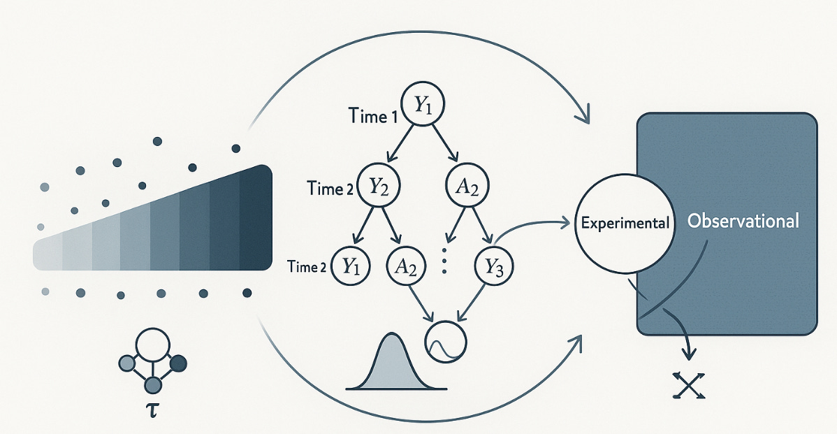
TL;DR: as more researchers rely on large observational datasets, a recurring issue emerges: these datasets capture rich outcomes and wide populations but lack randomisation (it turns out that even with larger Ns you still *do* need randomisation). At the same time, smaller experiments offer clean causal identification but only for a narrow set of outcomes or people. In this paper the authors introduce the Experimental Selection Correction (ESC) estimator, a way to use the experimental data to estimate and correct the bias in observational estimates. Think of it as training a correction function on the experiment, then applying it to the observational data. It’s a modern rethinking of Heckman-style selection correction, but with fewer assumptions and better performance when combined with ML tools.
What is this paper about?
There is a common, real-world, problem many of us applied researchers face: there is have an experiment, but it’s small or limited in scope; there’s also a big observational dataset, but it’s potentially biased. How do we combine them to get accurate causal estimates? Profs Athey, Chetty, and Imbens propose the Experimental Selection Correction (ESC) estimator, which uses the experimental data to learn the selection bias in the observational estimates, and then corrects for that bias across the broader sample. Their set-up is: in the observational data, one observes treatment and a wide set of outcomes, but treatment is not random, whereas in the experimental data, treatment is randomly assigned, but outcomes are more limited or less representative. Their key idea is: if one can measure the difference between the experimental and observational estimates for units observed in both, one can estimate a bias function. Then one can use that function to correct the observational estimates in the larger dataset. Mathematically, it’s similar in spirit to Heckman’s selection model, but the correction term is learned from experimental data rather than assumed from a structural model.
What do the authors do?
Profs Athey, Chetty, and Imbens introduce the Experimental Selection Correction (ESC) estimator, which adjusts observational treatment effect estimates using experimental data. We even have a DAG to exemplify the idea:
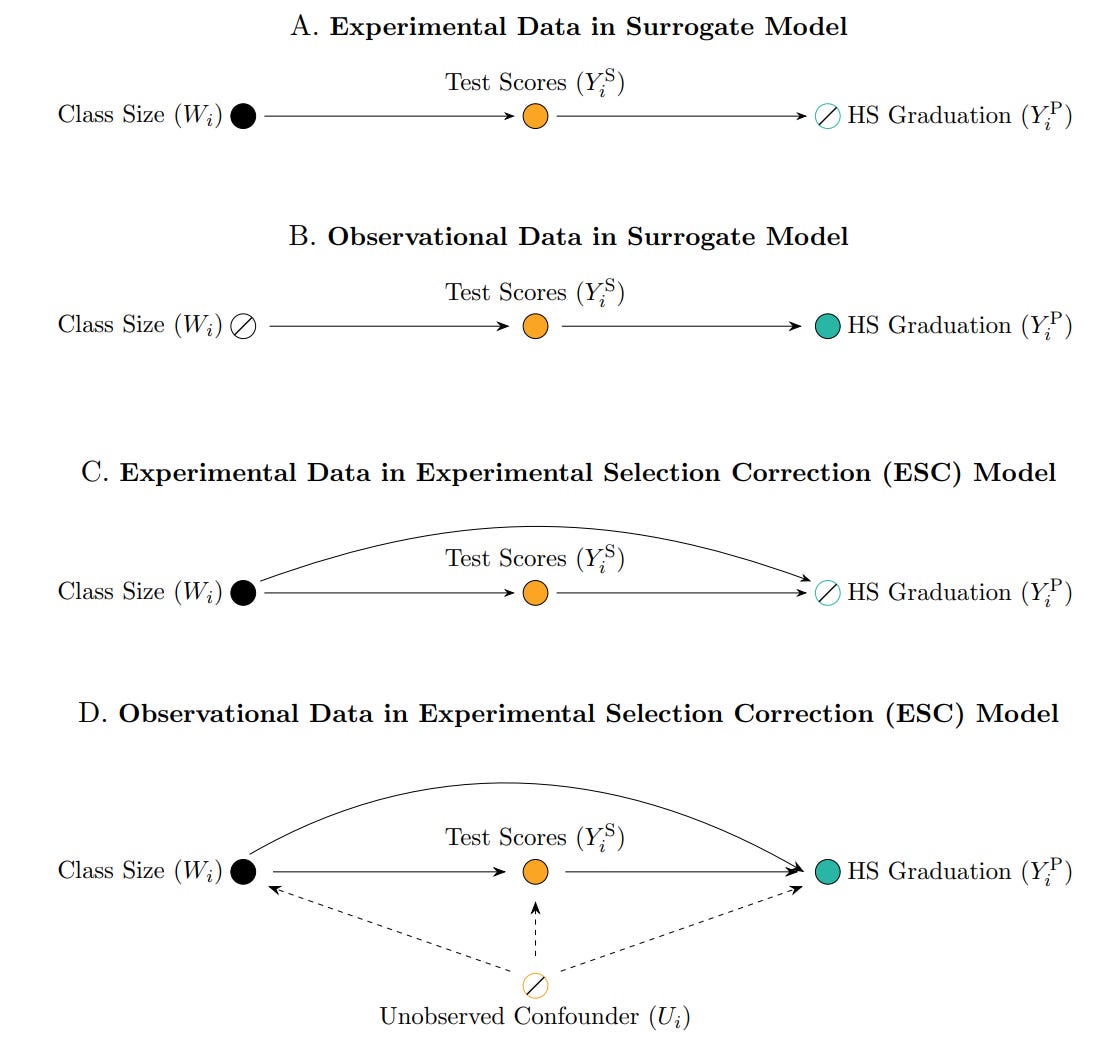
As one can see from the illustration, they build on the surrogate model literature, where researchers estimate the effect of a treatment on a surrogate outcome (like test scores), and then use the observed relationship between the surrogate and a long-term outcome (like graduation rates) to back out the treatment effect. This approach has been influential (Athey et al., 2019), but it assumes no unobserved confounding, which is an assumption often violated in observational settings. The ESC estimator extends the surrogate approach by explicitly modelling and correcting the bias in the observational estimates of long-term outcomes. It works in a few steps: you use the experimental sample (where treatment is randomly assigned) to estimate the bias in observational treatment effect estimates (i.e. the difference between experimental and observational effects, conditional on covariates); then you estimate a bias function (possibly using ML), that maps observed covariates to the size of the bias; and finaly you apply this bias correction to the observational sample to get a debiased treatment effect estimate. Then we can use a the large, rich observational dataset (but with bias removed) effectively combining the precision and scale of big data with the credibility of randomised experiments.
Why is this important?
There's this tweet that went viral once which reflects a common misconception that -especially in the era of Big Data - if your sample is large enough, you don’t need randomisation. But this paper flips that idea on its head. The authors show that selection bias doesn’t vanish with more data, it just becomes more precisely wrong. You can collect all the observational data in the world, but if treatment assignment is biased, the resulting estimate will be too. That’s why this paper matters. It offers a way to quantify and remove that bias using a well-designed experiment, even if the experiment is small or doesn’t cover every outcome. The idea is to enhance observational data for causal inference by using experimental insights to correct its flaws, thereby avoiding the need for complete replacement. It’s a flexible, scalable solution that keeps the credibility of experiments while unlocking the scope of big data.
Who should care?
This is for researchers who:
Work with large observational datasets (e.g. admin data, education records, firm-level panels)
Have access to some experimental variation, but not at the scale or granularity they need
Worry about selection bias but don’t want to rely on strong structural assumptions
Use ML for causal inference, but want a method that won’t be too difficult to justify when someone asks in a seminar
Do we have code?
We have an entire repo (in R) dedicated to it.
In summary, this paper delivers a powerful message: randomisation is still useful, even in the age of Big Data. Profs Athey, Chetty, and Imbens show how you can use experimental evidence to identify effects, as well as to repair the observational ones. Instead of throwing out observational data or blindly trusting it, their estimator lets you calibrate it. You borrow just enough credibility from the experiment to subtract out the bias, and then scale up your estimates with confidence. It’s a modern take on selection correction, grounded in theory but ready for real-world data.
Latent variables within a state-space structure means that the treatment effects aren’t directly observed or estimated from a single regression equation. Instead, they’re treated as unobserved time series that evolve over time according to a probabilistic process. The model uses the observed data to infer these hidden values step by step, borrowing information across time and units.